

Transport Assistant (TA) Experiment Guide
This guide describes how to evaluate the performance benefits of a Transport Assistant (TA) network function that caches and proactively retransmits packets to improve TCP performance in wireless environments. It provides a Mininet/Floodlight testbed for comparing plain TCP (Baseline) with the Transport Assistant, along with all the code, scripts, and instructions required to reproduce the experiments and generate the figures presented in the following publications:
- M. F. Zhani, R. Boughamoura, H. Yahyaoui, J. Kaippallimalil, and A. Kiani, “Oblivious TCP Support A Virtual Network Function to Speed Up TCP in Wireless Environments,” in IFIP Wireless and Mobile Networking Conference (WMNC), 2022, pp. 75–79. [PDF, BibTex]
- M. F. Zhani and H. Elbakoury, "FlexNGIA: A Flexible Internet Architecture for the Next‑Generation Tactile Internet," Journal of Network and Systems Management, Springer 2020. [PDF, PPT, BibTex]
1. Overview
This project evaluates a Transport Assistant (TA): a Netwok Function sitting between a client host (h1) and a server host (h2) that caches in-flight TCP segments and can retransmit them on the source's behalf to shorten recovery time after packet loss. Each experiment compares two conditions:
- Baseline: plain TCP with no TA involved
- TA: the same topology, but the TA node actively caches and retransmits
Results are logged as CSVs by each host during the run, then post-processed into comparison plots (flow completion time, per-packet RTT, retransmission counts, cache occupancy, throughput).
2. Prerequisites
- Download a this pre-installed VM using this link. This VM includes the following:
- Mininet: SDN emulator
- Floodlight controller installed at /home/floodlight-1.2/, built with ant (target/floodlight.jar must exist)
- Everything run as root: Mininet needs raw sockets and network-namespace access
- Requires jq, gnuplot, and the pre-built transpose binary (source in transpose.c to rebuild it if needed).
- Download the project: Download the complete project, including all the code required to run the experiments (TA, Mininet scripts, and figure generation scripts), using this link.
- Copy the project: Extract the downloaded archive and copy the entire project directory to /home/mininet, as the paths in the execution scripts are hardcoded to this location.
3. Running an Experiment, Step by Step
Step 1: Start the SDN controller
In a terminal, run:
sudo ./runController.sh
This command terminates any running Java processes and starts the
Floodlight SDN controller by executing
java -jar target/floodlight.jar.
Once the controller is running, the Open vSwitch switches created by
Mininet automatically connect to it on port 6653.
Step 2: Build the network topology
In a second terminal, run:
sudo ./runMininet.sh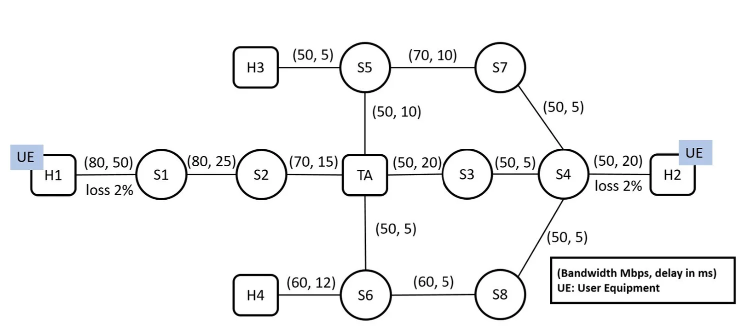
This command executes InfrastructureB.py, which builds the simulated
network topology (Figure 1). The topology consists of eight SDN switches, four hosts
(h1–h4), and the Transport Assistant (TA) node.
Each link is configured with predefined bandwidth, delay, and packet-loss
characteristics (for example, the link between h1 and
s1 is configured with 80 Mbps bandwidth, 50 ms delay, and 2% packet loss).
The TA node is configured with four network interfaces
(TA-eth0–TA-eth3), one for each subnet, and IP forwarding
is enabled so it can route traffic between the four subnets.
After the topology is created, the script opens the Mininet CLI
(the prompt appears as mininet>). The network remains active until
you exit the Mininet CLI.
Open terminals on the hosts: From the Mininet CLI, open xterm windows for the required hosts by running:
mininet> xterm h1 h2 TA
This command opens three xterm windows: one attached to
h1, one to h2, and one to the TA host.
Each xterm runs inside the corresponding host's network namespace,
so the commands executed in that terminal only see the interfaces,
routes, and processes of that host.
Step 3: Run each role, in order
-
In the h2 xterm (server), run:
./runServer.shThis command launches
clientStat.pyin the background for logging, then startsserverBaseline.pylistening on port47121. -
In the TA xterm (only for the TA experiment; skip this step for a Baseline run), run:
./runTA.shThis command runs
clientStat.py -o TA --cache -l TA-eth1 --rint0 TA-eth1 -a, which puts the TA into cache + proactive retransmission mode on the interface facingh2. -
In the h1 xterm (client), start the client last:
./runClient.shThis command starts
clientStat.pyfor logging, and then runsclientRetBaseline.py 10.0.2.10 47121to generate traffic to the server.
Each role writes its own CSV files:
ResultsTAClient.csv,
ResultsTAServer.csv,
ResultsTATA.csv,
the corresponding ResultsTATime*.csv time-series files,
and ResultsServerReport.csv.
For a Baseline run, place these files in
Results/Baseline/;
for a TA run, place them in
Results/TA/.
The script genFigures.sh expects exactly this directory layout.
Step 4: Repeat for both conditions (TCP with and without theTA)
Run the full Step 3 sequence twice:
- Once without starting the TA → move the resulting CSVs into Results/Baseline/
- Once with the TA running → move the resulting CSVs into Results/TA/
Step 5: Generate the comparison figures
cd Results
./genFigures.sh
This script:
- Builds a side-by-side Flow Completion Time (FCT) comparison from both experiments
(using File ResultsServerReport.csv) - Extracts specific fields (retransmissions, RTT sums) using the compiled ./transpose helper
- Feeds the processed data to gnuplot via the .gp scripts (FCTGnuOnline.gp, SrcRetGnu.gp, FRTT.gp, UnnRet.gp, OverTime.gp, etc.)
Output lands in Results/Figures/. Figures for the following metrics are generated (each comparing Baseline vs TA):
- Flow Completion Time
- FRTT (per-packet RTT which includes retransmission time)
- Unneeded retransmission counts
- Cache size (MB / packets) over time
- Send/receive rate in Mbps and pps
Step 6: Archive a run
To archive the entire experiment, including the scripts and the generated results, run:
./backup.sh all v2
This command creates a compressed archive containing the complete project,
including the Results/ directory, and stores it in the
Backup/ directory using a timestamped filename of the form
<timestamp>-TA-allv2.tgz.
To archive only the source code and figure-generation scripts (without the experimental data), run:
./backup.sh code v2This command creates a compressed archive containing the project source code and the Gnuplot scripts, but excludes the experimental results.